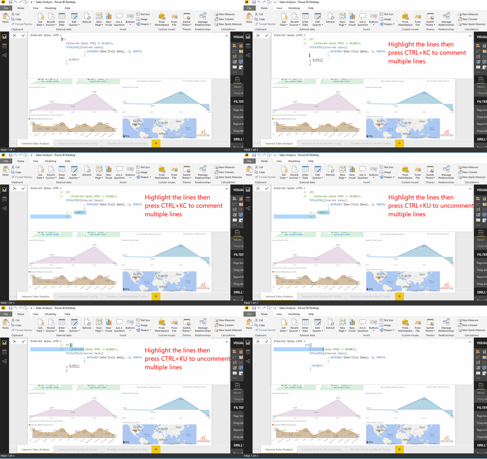
There are lots of cases you may want to comment/uncomment multiple lines in DAX scripts. You can save lots of development time if you know the shortcuts.
Here you go:
- Select multiple lines of code you want to comment
- Press Crtl+KC to comment those lines
- Press Ctrl+KU to uncomment commented lines

Mini-tip: The shortcuts work in SQL Server Management Studio (SSMS) writing any queries including DAX queries.
Enjoy!
Discover more from BI Insight
Subscribe to get the latest posts sent to your email.
I am feeling motivated and now work harder to start the career in Power-BI, hope will get similar success. Thanks for sharing your Power-BI experience.
what is KU?
On your keyboard, press Ctrl, K and while still pressing Ctrl, press U.
Hopefully that clearer now.
Hi hoping you can help. I’m trying to use the IMPORTRANGE function, but to pull across a value based on a formula from another spreadsheet, rather than choosing a specific cell.For example I have this formula on another spreadsheet:=large(‘Chester Data’!E7:E172,1)Which gives me the highest value within the range E7:E172 and returns this as a value into the cell with the formula in.What I want is it to do this between spreadsheets, though if I put the formula above in my IMPORTRANGE is obviously doesn’t work as the value the formula gives isn’t a cell reference, which is what the IMPORTRANGE needs.So basically I need a formula that returns a cell reference based on a cell contents, I could then run this formula on the above LARGE formula, give me a specific cell on the first spreadsheet and then IMPORTRANGE this to the next spreadsheet.Hope that makes sense …
Hi Sanford,
Welcome to biinsight.com, and thanks for sharing the challenge you are facing.
Unfortunately, I am not an Excel expert, but I am sure many of my website visitors, like yourself, are.
So perhaps you get some advice from others.
Cheers.
Certainly! To achieve this, you can use a combination of the `INDEX` and `MATCH` functions along with `IMPORTRANGE`. Here’s a step-by-step guide:
Assuming you have the formula `=LARGE(‘Chester Data’!E7:E172, 1)` in another spreadsheet, and you want to import the value from the cell with the maximum value in that range to a different spreadsheet using `IMPORTRANGE`, you can follow these steps:
1. On the source spreadsheet (‘Chester Data’ in this case), create a helper column to store the row number of the maximum value. You can use the following formula in, let’s say, column F:
“`excel
=MATCH(LARGE(‘Chester Data’!E7:E172, 1), ‘Chester Data’!E7:E172, 0) + 6
“`
This formula finds the position of the maximum value in the range E7:E172 and adds 6 (assuming your data starts from row 7).
2. Now, you can use the `INDEX` function to get the value from the cell corresponding to the maximum value. In another cell, you can use:
“`excel
=INDEX(‘Chester Data’!E7:E172, MATCH(LARGE(‘Chester Data’!E7:E172, 1), ‘Chester Data’!E7:E172, 0))
“`
This formula retrieves the actual value corresponding to the maximum value.
3. Now, in your destination spreadsheet, you can use `IMPORTRANGE` to bring this value:
“`excel
=IMPORTRANGE(“spreadsheet_key”, “Sheet1!A1”) // Replace “spreadsheet_key” with the key of the source spreadsheet and adjust the cell reference accordingly.
“`
Replace “spreadsheet_key” with the actual key of your source spreadsheet, and adjust the sheet and cell references based on your data.
Following these steps, you should be able to import the value from the cell with the maximum value in the specified range from one spreadsheet to another using `IMPORTRANGE`.