
When I decided to write this blog post, I thought it would be a good idea to learn a bit about the history of Business Intelligence. I searched on the internet, and I found this page on Wikipedia. The term Business Intelligence as we know it today was coined by an IBM computer science researcher, Hans Peter Luhn, in 1958, who wrote a paper in the IBM Systems journal titled A Business Intelligence System as a specific process in data science. In the Objectives and principles section of his paper, Luhn defines the business as “a collection of activities carried on for whatever purpose, be it science, technology, commerce, industry, law, government, defense, et cetera.” and an intelligence system as “the communication facility serving the conduct of a business (in the broad sense)”. Then he refers to Webster’s dictionary’s definition of the word Intelligence as “the ability to apprehend the interrelationships of presented facts in such a way as to guide action towards a desired goal”.
It is fascinating to see how a fantastic idea in the past sets a concrete future that can help us have a better life. Isn’t it precisely what we do in our daily BI processes as Luhn described of a Business Intelligence System for the first time? How cool is that?
When we talk about the term BI today, we refer to a specific and scientific set of processes of transforming the raw data into valuable and understandable information for various business sectors (such as sales, inventory, law, etc…). These processes will help businesses to make data-driven decisions based on the existing hidden facts in the data.
Like everything else, the BI processes improved a lot during its life. I will try to make some sensible links between today’s BI Components and Power BI in this post.
Generic Components of Business Intelligence Solutions #
Generally speaking, a BI solution contains various components and tools that may vary in different solutions depending on the business requirements, data culture and the organisation’s maturity in analytics. But the processes are very similar to the following:
- We usually have multiple source systems with different technologies containing the raw data, such as SQL Server, Excel, JSON, Parquet files etc…
- We integrate the raw data into a central repository to reduce the risk of making any interruptions to the source systems by constantly connecting to them. We usually load the data from the data sources into the central repository.
- We transform the data to optimise it for reporting and analytical purposes, and we load it into another storage. We aim to keep the historical data in this storage.
- We pre-aggregate the data into certain levels based on the business requirements and load the data into another storage. We usually do not keep the whole historical data in this storage; instead, we only keep the data required to be analysed or reported.
- We create reports and dashboards to turn the data into useful information
With the above processes in mind, a BI solution consists of the following components:
- Data Sources
- Staging
- Data Warehouse/Data Mart(s)
- Extract, Transform and Load (ETL)
- Semantic Layer
- Data Visualisation
Data Sources #
One of the main goals of running a BI project is to enable organisations to make data-driven decisions. An organisation might have multiple departments using various tools to collect the relevant data every day, such as sales, inventory, marketing, finance, health and safety etc.
The data generated by the business tools are stored somewhere using different technologies. A sales system might store the data in an Oracle database, while the finance system stores the data in a SQL Server database in the cloud. The finance team also generate some data stored in Excel files.
The data generated by different systems are the source for a BI solution.
Staging #
We usually have multiple data sources contributing to the data analysis in real-world scenarios. To be able to analyse all the data sources, we require a mechanism to load the data into a central repository. The main reason for that is the business tools required to constantly store data in the underlying storage. Therefore, frequent connections to the source systems can put our production systems at risk of being unresponsive or performing poorly. The central repository where we store the data from various data sources is called Staging. We usually store the data in the staging with no or minor changes compared to the data in the data sources. Therefore, the quality of the data stored in the staging is usually low and requires cleansing in the subsequent phases of the data journey. In many BI solutions, we use Staging as a temporary environment, so we delete the Staging data regularly after it is successfully transferred to the next stage, the data warehouse or data marts.
If we want to indicate the data quality with colours, it is fair to say the data quality in staging is Bronze.
Data Warehouse/Data Mart(s) #
As mentioned before, the data in the staging is not in its best shape and format. Multiple data sources disparately generate the data. So, analysing the data and creating reports on top of the data in staging would be challenging, time-consuming and expensive. So we require to find out the links between the data sources, cleanse, reshape and transform the data and make it more optimised for data analysis and reporting activities. We store the current and historical data in a data warehouse. So it is pretty normal to have hundreds of millions or even billions of rows of data over a long period. Depending on the overall architecture, the data warehouse might contain encapsulated business-specific data in a data mart or a collection of data marts. In data warehousing, we use different modelling approaches such as Star Schema. As mentioned earlier, one of the primary purposes of having a data warehouse is to keep the history of the data. This is a massive benefit of having a data warehouse, but this strength comes with a cost. As the volume of the data in the data warehouse grows, it makes it more expensive to analyse the data. The data quality in the data warehouse or data marts is Silver.
Extract, Transfrom and Load (ETL) #
In the previous sections, we mentioned that we integrate the data from the data sources in the staging area, then we cleanse, reshape and transform the data and load it into a data warehouse. To do so, we follow a process called Extract, Transform and Load or, in short, ETL. As you can imagine, the ETL processes are usually pretty complex and expensive, but they are an essential part of every BI solution.
Semantic Layer #
As we now know, one of the strengths of having a data warehouse is to keep the history of the data. But over time, keeping massive amounts of history can make data analysis more expensive. For instance, we will have a problem if we want to get the sum of sales over 500 million rows of data. So, we pre-aggregate the data into certain levels based on the business requirements into a Semantic layer to have an even more optimised and performant environment for data analysis and reporting purposes. Data aggregation dramatically reduces the data volume and improves the performance of the analytical solution.
Let’s continue with a simple example to better understand how aggregating the data can help with the data volume and data processing performance. Imagine a scenario where we stored 20 years of data of a chain retail store with 200 stores across the country, which are open 24 hours and 7 days a week. We stored the data at the hour level in the data warehouse. Each store usually serves 500 customers per hour a day. Each customer usually buys 5 items on average. So, here are some simple calculations to understand the amount of data we are dealing with:
- Average hourly records of data per store: 5 (items) x 500 (served cusomters per hour) = 2,500
- Daily records per store: 2,500 x 24 (hours a day) = 60,000
- Yearly records per store: 60,000 x 365 (days a year) = 21,900,000
- Yearly records for all stores: 21,900,000 x 200 = 4,380,000,000
- Twenty years of data: 4,380,000,000 x 20 = 87,600,000,000
A simple summation over more than 80 billion rows of data would take long to be calculated. Now, imagine that the business requires to analyse the data on day level. So in the semantic layer we aggregate 80 billion rows into the day level. In other words, 87,600,000,000 ÷ 24 = 3,650,000,000 which is a much smaller number of rows to deal with.
The other benefit of having a semantic layer is that we usually do not require to load the whole history of the data from the data warehouse into our semantic layer. While we might keep 20 years of data in the data warehouse, the business might not require to analyse 20 years of data. Therefore, we only load the data for a period required by the business into the semantic layer, which enhances the overall performance of the analytical system.
Let’s continue with our previous example. Let’s say the business requires analysing the past 5 years of data. Here is a simplistic calculation of the number of rows after aggregating the data for the past 5 years at the day level: 3,650,000,000 ÷ 4 = 912,500,000.
The data quality of the semantic layer is Gold.
Data Visualisation #
Data visualisation refers to representing the data from the semantic layer with graphical diagrams and charts using various reporting or data visualisation tools. We may create analytical and interactive reports, dashboards, or low-level operational reports. But the reports run on top of the semantic layer, which gives us high-quality data with exceptional performance.
How Different BI Components Relate #
The following diagram shows how different Business Intelligence components are related to each other:
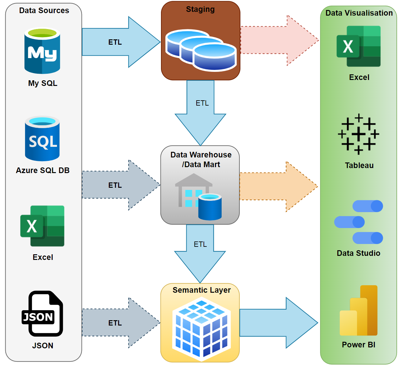
In the above diagram:
- The blue arrows show the more traditional processes and steps of a BI solution
- The dotted line grey(ish) arrows show more modern approaches where we do not require to create any data warehouses or data marts. Instead, we load the data directly into a Semantic layer, then visualise the data.
- Depending on the business, we might need to go through the orange arrow with the dotted line when creating reports on top of the data warehouse. Indeed, this approach is legitimate and still used by many organisations.
- While visualising the data on top of the Staging environment (the dotted red arrow) is not ideal; indeed, it is not uncommon that we require to create some operational reports on top of the data in staging. A good example is creating ad-hoc reports on top of the current data loaded into the staging environment.
How Business Intelligence Components Relate to Power BI #
To understand how the BI components relate to Power BI, we have to have a good understanding of Power BI itself. I already explained what Power BI is in a previous post, so I suggest you check it out if you are new to Power BI. As a BI platform, we expect Power BI to cover all or most BI components shown in the previous diagram, which it does indeed. This section looks at the different components of Power BI and how they map to the generic BI components.
Power BI as a BI platform contains the following components:
- Power Query
- Data Model
- Data Visualisation
Now let’s see how the BI components relate to Power BI components.
ETL: Power Query #
Power Query is the ETL engine available in the Power BI platform. It is available in both desktop applications and from the cloud. With Power Query, we can connect to more than 250 different data sources, cleanse the data, transform the data and load the data. Depending on our architecture, Power Query can load the data into:
- Power BI data model when used within Power BI Desktop
- The Power BI Service internal storage, when used in Dataflows
With the integration of Dataflows and Azure Data Lake Gen 2, we can now store the Dataflows’ data into a Data Lake Store Gen 2.
Staging: Dataflows #
The Staging component is available only when using Dataflows with the Power BI Service. The Dataflows use the Power Query Online engine. We can use the Dataflows to integrate the data coming from different data sources and load it into the internal Power BI Service storage or an Azure Data Lake Gen 2. As mentioned before, the data in the Staging environment will be used in the data warehouse or data marts in the BI solutions, which translates to referencing the Dataflows from other Dataflows downstream. Keep in mind that this capability is a Premium feature; therefore, we must have one of the following Premium licenses:
Data Marts: Dataflows #
As mentioned earlier, the Dataflows use the Power Query Online engine, which means we can connect to the data sources, cleanse, transform the data, and load the results into either the Power BI Service storage or an Azure Data Kale Store Gen 2. So, we can create data marts using Dataflows. You may ask why data marts and not data warehouses. The fundamental reason is based on the differences between data marts and data warehouses which is a broader topic to discuss and is out of the scope of this blogpost. But in short, the Dataflows do not currently support some fundamental data warehousing capabilities such as Slowly Changing Dimensions (SCDs). The other point is that the data warehouses usually handle vast volumes of data, much more than the volume of data handled by the data marts. Remember, the data marts contain business specific data and do not necessarily contain a lot of historical data. So, let’s face it; the Dataflows are not designed to handle billions or hundred millions of rows of data that a data warehouse can handle. So we currently accept the fact that we can design data marts in the Power BI Service using Dataflows without spending hundreds of thousands of dollars.
Semantic Layer: Data Model or Dataset #
In Power BI, depending on the location we develop the solution, we load the data from the data sources into the data model or a dataset.
Using Power BI Desktop (desktop application)
It is recommended that we use Power BI Desktop to develop a Power BI solution. When using Power BI Desktop, we directly use Power Query to connect to the data sources and cleanse and transform the data. We then load the data into the data model. We can also implement aggregations within the data model to improve the performance.
Using Power BI Service (cloud)
Developing a report directly in Power BI Service is possible, but it is not the recommended method. When we create a report in Power BI Service, we connect to the data source and create a report. Power BI Service does not currently support data modelling; therefore, we cannot create measures or relationships etc… When we save the report, all the data and the connection to the data source are stored in a dataset, which is the semantic layer. While data modelling is not currently available in the Power BI Service, the data in the dataset would not be in its cleanest state. That is an excellent reason to avoid using this method to create reports. But it is possible, and the decision is yours after all.
Data Visualisation: Reports #
Now that we have the prepared data, we visualise the data using either the default visuals or some custom visuals within the Power BI Desktop (or in the service). The next step after finishing the development is publishing the report to the Power BI Service.
Data Model vs. Dataset
At this point, you may ask about the differences between a data model and a dataset. The short answer is that the data model is the modelling layer existing in the Power BI Desktop, while the dataset is an object in the Power BI Service. Let us continue the conversation with a simple scenario to understand the differences better. I develop a Power BI report on Power BI Desktop, and then I publish the report into Power BI Service. During my development, the following steps happen:
- From the moment I connect to the data sources, I am using Power Query. I cleanse and transform the data in the Power Query Editor window. So far, I am in the data preparation layer. In other words, I only prepared the data, but no data is being loaded yet.
- I close the Power Query Editor window and apply the changes. This is where the data starts being loaded into the data model. Then I create the relationships and create some measures etc. So, the data model layer contains the data and the model itself.
- I create some reports in the Power BI Desktop
- I publish the report to the Power BI Service
Here is the point that magic happens. During publishing the report to the Power BI Service, the following changes apply to my report file:
- Power BI Service encapsulates the data preparation (Power Query), and the data model layers into a single object called a dataset. The dataset can be used in other reports as a shared dataset or other datasets with composite model architecture.
- The report is stored as a separated object in the dataset. We can pin the reports or their visuals to the dashboards later.
There it is. You have it. I hope this blog post helps you better understand some fundamental concepts of Business Intelligence, its components and how they relate to Power BI. I would love to have your feedback or answer your questions in the comments section below.
Discover more from BI Insight
Subscribe to get the latest posts sent to your email.